Machine Learning Notes 06

How biological neural network work

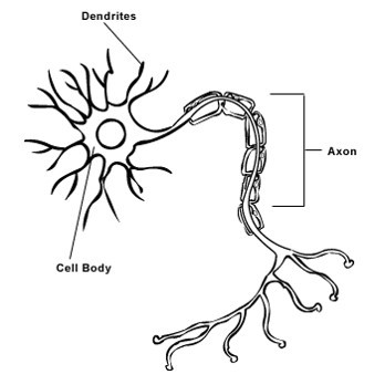
  As the following image shown, there are three main parts in each neuron: Dendrites, Cell Body and Axon. The signals come from the last neuron to the dendrites first, then enter into the cell body. While the potential would be judged with the threshold and then output the signals into the axon, that’s approximately how biological nerual network run.

How artificial neural network work

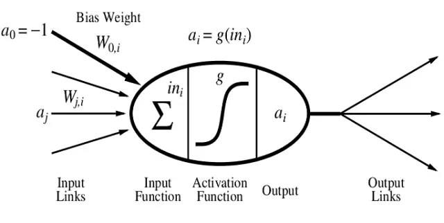
  The pictures above shows a basic unit of the artificial nerual network, we usually call it as perceptron, which you can consider it as the neuron of the neural network. It works similarly as the biological neural network. The input data \(a_i\) was summed with the weights \(\omega\) , and then input the summing value and the threshold into the Activation Function, then we get the output value. We often choose the function \( g(z)=\frac{1}{1+e^{-z}} \) as our activation function. Then we return the bias back to adjust the parameters (weights \(\omega\)), when the parameters converge, the learning process end.

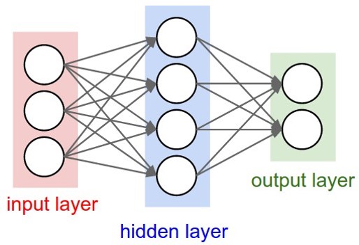
  And here’s what a three-layer ann looks like,

  The first layer, which is the input data belong to, is called Input Layer, while the last layer is called as Output Layer which is used to ouput data. And layer(s) in the middle of the input layer and output layer is called Hidden Layer, and the quantities of the hidden layers can be 1, 2, 3, …, even hundreds or thousands. the more hidden layers a neural network have, the more complex the system would be, which causes the calculation more difficult (and that’s why we need more).

Feedforward Propagation Algorithm

  We obtain the output first, by: \(y_{j}=g(\sum^{n}_{i=1}\omega_{ji}x_i-\theta),\)

,and we often choose sigmoid function \(g(z)=\frac{1}{1+e^{-z}}\) as our activation function. For the more complex situation, we can also use vectorization:

\(a_{n+1}=g(a_{n}*\Theta_n)\)

(\(a_n\) stands for the input in the \(n^{th}\) layer)

Back Propagation Algorithm

For the training set \({(x^{(1)},y^{(1)}),\cdots,(x^{(m)},y^{(m)}) }\), \(\Delta_{ij}^{(l)}=0 \) (for all \(l,i,j\)). Then we run the following loop:

For \(i = 1\) to \(m\):

　　Set \(a^{(1)}=x^{(i)}\)

　　Perform forward propagation to compute \(a^{(l)}\) for \(l=2,3,..,L\)

　　Using \(y^{(i)}\), compute \(\delta^{L}=a^{(L)}-y^{(i)}\)

　　Compute \(\delta^{(L-1)}, \delta^{(L-2)}, \cdots, \color{red}{\delta^{(2)}}\)

　　\( \Delta_{ij}^{(l)}:=\Delta_{ij}^{(l)} + a^{(l)}{j}\delta^{l+1}{i} \)

After that,

　　\(D_{ij}^{(l)}:= \frac{1}{m}\Delta_{ij}^{(l)}+ \lambda\Theta^{(l)}_{ij}\) if \(j\neq0\)

　　\(D_{ij}^{(l)}:= \frac{1}{m}\Delta_{ij}^{(l)}\)　 if \(j=0\)

And we get:

　　\(\frac{\partial}{\partial\Theta^{(l)}_{ij}}J(\Theta) = D_{ij}^{(l)}\)

Process of Training a Neural Network

1. Randomly initialize the weights;
2. Implement forward propagation to get \(h_{\Theta}(x^{(i)})\) for any \(x^{(i)}\);
3. Implement the cost function;
4. Implement backpropagation to compute partial derivatives;
5. Use gradient checking to confirm that your backpropagation works. Then disable gradient checking;
6. Use gradient descent or a built-in optimization function to minimize the cost function with the weights in theta;